MSc thesis: Leveraging APL and SPIR-V languages to
write network functions to be deployed on Vulkan compatible GPUs
Abstract
Present-day computers apply parallelism for high throughput and low
latency calculations. However, writing of performant and concise
parallel code is usually tricky.
In this study, we tackle the problem by compromising on programming
language generality in favor of conciseness. As a novelty, we do this by
limiting the language’s data structures to rank polymorphic arrays. We
apply our approach to the domain of Network Function Virtualization
(NFV). We use GPUs as the target hardware. This complements NFV research
in replacing purpose-built hardware with commodity hardware. Further, we
present an empirical case study of a random forest implementation used
to classify network traffic. We write the application for GPUs with
SPIR-V Intermediate Representation (IR) while using APL as a modeling
language.
To our knowledge, this approach is novel in three ways. First, SPIR-V
has not yet been demonstrated to be used in machine learning
applications. Second, we translate a non-imperative language APL to
SPIR-V GPU IR. Using a non-imperative source language for GPUs is rare
in general. Third, we show how SPIR-V programs can be used in Kubernetes
microservice orchestration system. This integrates our proposed parallel
computation pipeline to industry NFV deployment standards.
We benchmark the SPIR-V code against C with a random forest of size
150x6000x300. We find 8-core CPU runtime to average 380ms and RTX 2080
GPU to average 480ms. Hence, space is left for further improvements in
future work, which we detail for both the GPU pipeline and APL to GPU
compilation.
Leveraging APL and SPIR-V languages to write network functions
to be deployed on Vulkan compatible GPUs
200(10,12) University of Lorraine Master of Computer
Science - MFLS Master’s Thesis Juuso Haavisto Supervisor: Dr.
Thibault Cholez Research Team: RESIST 1980-01-01
Introduction
In the software industry, progress in computation capability has
historically followed Moore’s law. While it is an open debate whether
Moore’s law still holds, it’s without a doubt that classical computer
architectures have evolved to multi-core. To elaborate, commodity
computers in the 20th century were single-core systems. This paradigm
saw a big change at the start of the 21st century. During the first
decade, the physical core count started to increase rapidly. First came
the dual-core processors: in 2001, IBM POWER4 became the first
commercially available multi-core microprocessor. Similarly, AMD
released their first dual-core system in 2005 under brand name
Athlon 64 X2, and Intel released Core Duo processor
series in 2006. Core count has then kept on steadily increasing on each
microprocessor release: in 2020, the flagship consumer multi-core
processor from AMD, called Ryzen Threadripper 3990X, has 64
physical cores and 128 logical threads. Moreover, in the GPU
landscape, the difference is even larger. E.g., in 2005 a Nvidia
flagship GPU model GeForce 6800 GT had 16 cores for pixel
shaders. In 2020, a GeForce RTX 2080 Ti sports 4352 shader
processors.
Yet, despite the hardware changing, most programmers still think of
software from the viewpoint of a single thread. Performance-wise this is
suboptimal, as it means that the way software benefits from multi-core
systems are dependant on the smartness of the compiler. Further, as
parallelism is abstracted from the programmer, it is easy to construct
data-and control-structures which result in execution logic that cannot
be safely parallelized, or parallelized without much performance gain
compared to single-core processing.
As such, an open research question remains: how parallel software
could be better programmed? Coincidentally, this is the topic of this
study. In particular, we focus on GPUs. GPUs
have recently found use as a general-purpose computation accelerator for
programs with high parallelisms, such as machine learning. Here, the
data structures of these programs tend to be based on arrays: languages
which encode software for GPUs, e.g., Futhark (Henriksen et al.
2017), is based on the purely functional array programming
paradigm. But, we take the array programming paradigm a step further,
inspired by APL(Hui and Kromberg 2020), which only
permits array data structures. To achieve such semantic in practice, we
translate our program into SPIR-V. SPIR-V is the current
technological spearhead of GPUSSAIRs. Our thesis is that by
combining the language and the execution environment to only match the
usual computation domain tackled with GPUs, we could better reason
about such programs. As such, this directly addresses the problem of
efficient use of current computation hardware. Should it be possible to
implicitly parallelize all computations while enforcing parallel program
construction, we could ensure that software runs as fast as physically
possible. To our knowledge, this is the first attempt at creating a
compute DSL on top of SPIR-V.
The study is organized as follows: first in §2, we present a
literature review. The review considers cloud computing models, and
programming language approaches to achieve parallelism. After this, we
move onto the empirical part in §3. First,
in §3.1, we select a machine learning
application written in Python and look at how it uses a C-language sub
interpreter to produce parallel code for CPUs. The selected machine
learning application considers NFV, i.e., use-case in which
machine learning models are used for network processing. The machine
learning application in question comes from a previous paper (Brissaud et al.
2019) of the research group under which this study was conducted.
Next, we manually translate its Python-and-C implementation into APL.
The APL code we then manually translate into SPIR-V. Some technical details
of the SPIR-V translation are presented in §3.2. Next, in
§3.3 we present the GPU
system architecture. In §3.3.1, we start with the high-level view of
how a Vulkan-based GPU bootloader. We describe
how the loader can be integrated as a microservice in today’s de-facto
industrial cloud computing framework called Kubernetes. The loader
program in itself, which leverages a systems programming language Rust
and a low-level Vulkan API to control the GPU,
is described in §3.3.2. After this, in §3.4 we benchmark the SPIR-V against the Python-C
implementation. This marks a performance comparison between a CPU and
GPU processing for the machine learning application. Yet, we concede to
the fact that the comparison is not evenly-leveled: the CPU is given a
headstart due to a small sample size. We consider this an acceptable
limitation in our research. This is because it contributes to a
tangential research question about whether latency-sensitive computing,
here, NFV, can be accelerated with
GPUs. Following the results, in
§4, we contribute our findings on how
our loader program and APL to SPIR-V compilation could be improved.
Finally, the study is concluded in §5.
Previous research
In the introduction, we pointed how computer programming has changed
in the past 20 years in the form of parallelity: multi-processor CPUs
have become ubiquitous, and GPUs are in increasing effect used for
highly parallel workloads in domains of machine learning, where
thousands of cores are used to solve tasks. Similarly, the way software
is architected and turned into consumer services has also changed. Early
worldwide web applications were widely architected as a client-server
model with so-called monolithic application architecture. Here,
monolithic applications mean that a single program did all possible
computations required by the service and was likely run on a single
dedicated server computer. While the client-server model has remained
the standard during this century1, architectures have seen
a proliferation towards microservices, which run in cloud computing
environments. Such microservices are globally distributed within the
cloud provider network, and provisioned inside resource isolated
containers (Burns et
al. 2016) and, as of more recently, inside virtual machines with
formal semantics (Haas et al. 2017;
Watt 2018). In general, computing can be seen to have higher
execution granularity than before, shifting from a single computer
execution towards distributed execution of highly parallelized
individual threads. For example, in (Fouladi et al. 2017), video
processing is split among thousands of tiny threads across many physical
servers. Similarly, the Ethereum project is an attempt at a so-called
world computer concept. In accordance with the microservice trend,
Ethereum has software "contracts," which are executed among multiple
computers to form a consensus of the world’s computer state. However,
both in Ethereum and in the cloud there exists open safety challenges:
it is 1) hard for programmers to formally reason about the distributed
execution of their code, and 2) it is hard to ensure that the scheduler
does not leak confidential data when resources are re-used (Jangda et al.
2019) or that the scheduler is fair.
It could be considered that software that is architected to be
distributed is called cloud-native. In the following subsections, we
further inspect different ways to comprise microservices that yield to
this concept.
Microservice Runtimes
Microservice, as a term, has a loose definition. For the sake of
simplicity, in our study, we do not consider the social aspects, but
instead how the definition changes depending on what the underlying
technical runtime is. To elaborate on the problem statement: a
microservice with a container runtime runs a whole operating system on
each container. As such, container-based microservices have very lax
technical limitations. This is because an operating system has many
processes, and in the end, a microservice will be a process. But this
introduces a problem. Since the operating system can essentially an
arbitrary amount of processes, a single container may be compromised of
multiple microservices. While an organization can decide that each
process that is not a vital operating system process is a microservice,
sometimes such an approach is impractical. For example, a program may
have a proprietary dependency that may not listen to network ports. In
this case, a process-based definition for a microservice would not
work.
In general, it could be considered that when a microservice runtime
is not restrictive, it becomes a social problem to define it. As the
following subsections will show, some technical approaches have emerged
which are more restrictive. Here, the program granularity is reduced
from the container’s process towards a lambda function. For the sake of
conciseness, we evaluate what we consider widely known approaches of
microservice runtimes, shown in Fig. [tb:runtimes].
Technology
Overhead
Application Capabilities
Orchestrator
VM
Full OS + Full OS
Full OS
e.g., Xen
Containers
Full OS + Partial OS
Full OS
Kubernetes (Burns et al. 2016)
Unikernels
Partial OS
Full OS
e.g., iPXE
Serverless
Full OS + WASM Runtime
A function
e.g., Lucet
Technology
DSL
Overhead
Application Capabilities
Orchestrator
GPUs
e.g., SPIR-V
Full OS + Graphics API + GPU
A chain of functions
e.g., Legate (Bauer and Garland 2019)
Linux kernel passthrough
e.g., BPF
Any deployment method on Linux
A chain of functions
FPGAs
e.g., P4
Specialized hardware
A chain of functions
Containers
Arguably the most well-known packaging format of software is
currently containers, which developers usually interface via Docker or
some other CRI. As containers focus on
isolation and dependency minimization of arbitrary software, it makes
them a compelling basis for microservices. In the abstract, the idea is
that the developer creates a reproducible and self-contained
build-script for their applications from a clean-slate operating system
installation. This way, the developer may install any software required
to run their application while also making a reproducible build system
that allows restarts and migrations of the container. Such features are
relevant, as containers nowadays often run with orchestration systems
such as Kubernetes (Burns et al. 2016). Such
orchestration systems claim to make managing containers to equal
managing applications rather than machines (Burns et al. 2016), simplifying
development operations, and pooling all computation capabilities into a
single uniform abstraction. Further, these abstractions enable the
software development process to be streamlined and simplified from the
viewpoint of the developer: in our previous studies, e.g., (Haavisto et al.
2019), a Kubernetes-based installation is coupled with a
version-control integrated deployment process. Such abstraction then
even abstracts away the whole concept of computing resources, which
might, in turn, help developers focus on business goals better.
Especially in the industry, a promise of a universal solution to deploy
software to production becomes compelling: according to (Burns et al. 2016),
containers isolate applications from operating systems, making them
possible to provide the same deployment environment in both development
and production, which, in turn, improves deployment reliability and
speeds up development by reducing inconsistencies and friction.
Generally, containers are lightweight and fast: a single server can
have hundreds of containers running (Amaral et al. 2015). Yet,
containers also produce overhead in the form of nested operation
systems. Such challenges are to be considered, especially for
performance-centric microservices architectures and, in our case,
intensive I/O processing from network interfaces. To elaborate, should
one rent a virtual server from a cloud provider such as Amazon, they
already operate above an abstraction as cloud providers tend to rent
only virtualized environments for customers. On top of this abstraction,
a container-based approach requires an installation of the so-called
host operating system (e.g., Ubuntu), on which the actual containers
(e.g., Alpine Linux) are run. As such, a containerized application can
quickly end up operating on top of three separate operating systems,
each having their overhead. This may be challenging, especially for
networking: one study concludes that containers decrease network
performance by about 10% to 20% compared to bare-metal (i.e., non-nested
container) deployments (Kratzke 2017).
Serverless
When it comes to modern microservice runtimes, the serverless
paradigm is the most recent and finer in granularity: here, the
packaging format is a single function instead of the whole operating
system. Such an approach has some interesting traits: it has
significantly less overhead than containers, which make serverless
applications much faster to respond to actions even if scheduled
just-in-time. For example, the Amazon Firecracker scheduler has boot
times of around 150ms (Agache et al. 2020) compared
to seconds that it might take for a container on Kubernetes to start.
The so-called fast cold-start time is relevant when thinking about more
distributed and performance-orientated microservice architecture: the
orchestrator may free memory and cycle capacity by turning off
serverless applications which are not receiving traffic. And as soon as
one receives a request, it can be started by almost imperceptible
boot-up time. From a pragmatic perspective, it is also cost-efficient: a
serverless application may sleep and start on-demand and also billed
that way.
Yet, some studies, such as (Hellerstein et al. 2018),
argue that the serverless paradigm is "one step forward, two steps
back." One argument concerns the packaging method, i.e., the IR, of
serverless applications: with containers, the Dockerfile became the
de-facto manifest format to declare container installations, which in
itself resemble bash scripts by almost one-to-one. Yet, with serverless
applications, it may be a bigger social problem to agree on how
functions should be written. This problem directly stems from the fact
that with containers, any language that can be installed on any
operating system works, but with serverless, the users will likely
become restricted on a single language. While there already exists
papers of envisions of what the serverless paradigm will become, e.g.,
(Jonas et al.
2019), we denote that language-independent IRs are
gaining a foothold in the industry in the form of Wasm(Haas et al.
2017). In abstract, Wasm remarks a general shift
from build-script approaches of packaging software towards a
compiler-driven approach, in which the compiler backend produces Wasm
code instead of architecture-dependent bytecode. Originally, Wasm
was engineered to create faster and more heterogeneous JavaScript, but
the paralleling usefulness as a non-hardware specific IR and
the requirement of such in the serverless paradigm is an apparent and
promising fit.
Unikernels
A stark difference to the abstraction-heavy container and serverless
approach is unikernels. Unikernels address both the performance pitfalls
of layered kerneling of containers and can be used to avoid restricted
language support of serverless by packaging software as Linux kernels
(Raza et al.
2019). For example, MirageOS (Imada 2018) supports only
application written in OCaml, whereas Rumprun [cite] is a reduced
version of NetBSD, and as such, supports NetBSD compatible programming
languages. In general, the unikernel approach means taking a constrained
application environment, and packaging it as a Linux kernel (Raza et al.
2019) while stripping away operating system capabilities
unnecessary to the program. Relevant to our use of microservices, this
also means that performance-wise, kernel-passthrough approaches such as
BPF are not required for
solely performance reasons, as the application already runs in
kernel-mode. Further, unikernels make applications generally faster by
running in privileged mode, as a lot of performance-degrading bagging,
which comes from Linux security architecture to support a safe
multi-user paradigm, is set aside. Considering the orchestration of
unikernels, i.e., the deployment on a scale, to our understanding, no
de-facto method exists, yet we see no reason why networked BIOS
bootloaders like netboot [cite] would not work.
Executing microservices on
GPU
Network-processing has also been researched to be accelerated using
GPUs, e.g., via PacketShader
(Han et al.
2010). Here, the idea follows that computation tasks that concede
well under the physical constraints of GPUs are offloaded to a GPU.
This so-called GPGPU paradigm has recently
found its foothold in the form of machine learning applications, where
especially neural networks concede well to the physical constraints of
GPUs, which include a limited
and relatively slow uniform memory and MapReduce-like state
synchronization. Hence, it can be concluded that in the grand scheme of
general computation paradigms, GPUs follow the general
direction of distributed state like container deployments
(MapReduce-like state synchronization) and also the thread-granular
parallelism principles of serverless applications (slow uniform memory
enforces parallelism), but here within a single physical component. As
such, GPUs can also be thought of as a
microservice runtime, especially given support from an orchestrator such
as Legate (Bauer and
Garland 2019).
Yet, historically the GPGPU standards and approaches
have been dispersed at best: it remains commonplace to still use shading
languages like GLSL, meant to display
graphics on a monitor, to be tricked into computing matrix algebra by
using a no-display-producing graphics pipelines. There also exists an
open standard API called OpenCL, meant
solely for computation workloads, but the standardization is not only
meant for GPUs, but also for CPUs and FPGAs. Further, some GPU
manufacturers, such as Nvidia, have a proprietary IR
like the PTX which is produced by
Nvidia’s CUDAAPI
and as a backend target by the LLVM compiler infrastructure
to offer generally the most performant GPGPU code available today.
However, PTX only works on Nvidia GPUs.
Coincidentally, this also means that programming models for GPUs
are also scattered: historically, the only options have been either open
standards like OpenCL C or GLSL, or then
manufacturer-specific languages like CUDA. Somewhat surprisingly,
the programming model of these most common GPGPU languages is imperative,
whereas it has been commonplace for CPUs to have DSLs
with formal foundations on concurrency primitives like communicating
sequential processes (Hoare 1978) on recent
languages for multi-core environments like Erlang or Go.
More recently, the open GPU standards working group
called Khronos, which is the organization behind GLSL
and OpenCL, among many other open initiatives in the GPU
space, has released GPGPU enablers to a new
cross-platform graphics API focused on performance,
called the Vulkan API. These new capabilities
include a cross-platform formally verified memory model called the
Vulkan memory model (further introduced in §3.2.2), and a
class of cross-platform SIMD operands for non-uniform
group operations called subgroups (further introduced in §3.2.1). Yet, the Vulkan API,
while released in 2016, has not seemingly become the leading API
so far in the GPGPU space, plausibly
affected by a design decision to only support a new open standard IR
called SPIR-V. As such, any application which wishes to adopt Vulkan’s
features would first need to update all the GPU
code to SPIR-V, which in practice is
done via cross-compilers which may not necessarily translate the most
performant code. Further, some of the features, such as the Vulkan
memory model was released as recently as September 2019. We deem it
likely that most translators will require more time to adopt. As such,
as a consistent memory model is paramount for deterministic computation
results, it can be considered no subject of wonder why the technology
adoption may have been slow. Finally, regarding microservices, a
previous paper of ours (Haavisto and Riekki 2020)
studied the Vulkan and SPIR-V powered GPGPU paradigm in light of
cold-start times and interoperability: it was found that the 99th
percentile for starting the same programs was 1.4ms for a COTS desktop GPU (Nvidia RTX
2080), and 4.3ms for ARM-based COTS
mobile SoC (Nvidia Jetson TX2). So,
in terms of cold-start times, this places a modern GPGPU microservice latency to
the similar ballpark as serverless applications hence significantly
faster than containers.
Hardware
acceleration for parallel computing
How programming languages and approaches for machine
learning are made faster: by removing generality and by compromising on
utmost performance. (Model inspired by (Brown et al.
2011))
When thinking about programming languages to develop microservices,
we can think of an abstraction shaped like a triangle, shown in Fig. 1. On the left, we can see how programming
languages are located in different parts of the triangle, portraying
their focus on solving problems. For example, C is considered general
and highly performant. However, C is not considered very productive
because it allows a class of bugs to happen, which are not possible in
other languages. On the other hand, scripting languages like Python,
which are oftentimes used in machine learning, are not very fast, but as
a plus have general problem domains and are arguably easy to program. On
the left side, we have languages that are not very general, i.e., they
require separate computing accelerator devices like GPUs to work, but
yet for that reason are easier to program for domain-specificity. Hence,
such languages can assume more about the programming style than in
CPU-languages. Further, GPU languages do not have filesystem, network,
or persistent storage access. As such, reasoning about accelerator
languages can be considered easier, as unpredictable sources of infinite
input and output, e.g., file descriptors, do not exist.
Yet, it is also noteworthy to recognize that many approaches exist in
accelerating the languages found from the bottom side of the triangle
can be "lifted." By lifting, we mean there exist approaches for these
languages which move them towards the center of the triangle. In our
concept, a language that is at the center of the triangle is considered
an ideal programming language. But how does this lifting work? In this
section, we focus on some of such approaches, namely 1) advanced vector
extensions, 2) general-purpose computing on graphics processing
units.
Advanced Vector Extensions
AVX can be considered the
general method of accelerating programming languages on today’s
hardware. AVX achieves this by only operating on a subset of programs,
which yield to SIMD instructions— in a sense,
considering Fig. 1, AVXs can be efficiently applied
when generality is cut down to only consist of array operations and
data-parallel data structures. Coincidentally, as a result of
domain-specificity of AVX on SIMD, the triangle gets sliced
from the angle of generality. In practice, this angle-slicing effect is
usually applied to languages through scientific computing libraries,
which essentially only include matrix algebra in them. For example, in
Python, the NumPy library is such a domain-restricted library.
Once a library like NumPy is used, what essentially happens is that a
sub interpreter or just-in-time compiler gathers the program calls,
which are compiled down to platform-specific bytecode. This produced
bytecode is then the format on which the SIMD instructions have been
applied. Yet, as the bytecode generation is platform-specific, libraries
like OpenMP exist. These abstractions aim to compile the code to run as
fast as possible regardless of the platform. In practice, most of these
libraries leverage the LLVM compiler project to
detect and interoperate on a single shared IR. As seen, e.g., in Numba
(Lam, Pitrou, and
Seibert 2015), the LLVM IR is useful because as in some cases, it
allows a single IR to be compiled to vector instruction accelerated
CPU and GPU
code.
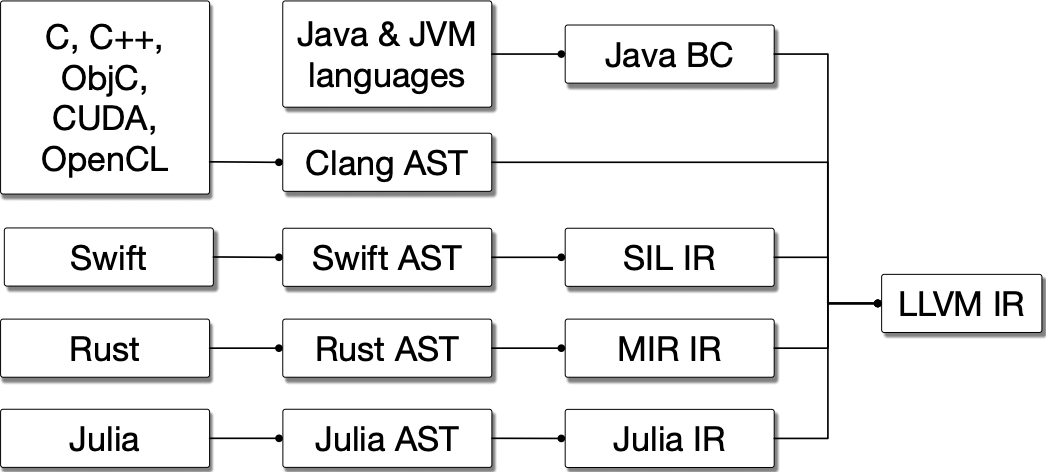
Compilation pipeline of different languages with multiple
mid-level IRs for language specific optimization with common backend for
multiple hardware targets. Source: (Lattner et al. 2020)
As of very recent, the power of shared IR and the shared compiler has
also been applied to domain-specific purposes itself, here, to deep
neural networks, as in MLIR (Lattner et al. 2020). As such, MLIR
can be considered a problem-domain specific SSA-based IR for heterogenous
target platforms, which include CPU, GPU, tensor programming unit (TPU),
and "others." We believe that this notion of compilers having more
features and compiler passes is interesting, as pictured in Fig. 2. That is, in recent languages like
Swift, Rust, and Julia, further compiler passes allow the developers to
write compiler extension libraries in the original language. In
specific, this mid-level pass is one that has passed the type-checker
but has not yet generated SSA code. As such, it seems generally
prosperous future development that the proliferation of more compiler
passes will help to move traditionally slow languages into faster ones
without any further input from the software developer.
In practice, we generalize those speed improvements are achieved by
effectively detecting code, which yields well to SIMD and
data-parallelism. Further, array-orientated libraries like NumPy
essentially function by exposing domain-specific pragmas to compilers,
which are often tacit to the software developer.
General-purpose computing on graphics processing
units
GPGPU is a similar approach as
AVX in the sense that GPGPU revolves around a similar register-based
programming style. However, this approach can be considered to be taken
even further: in the GPGPU paradigm, the software is essentially written
from the viewpoint of a single register. For example, in GPGPU, a vector
sum is something like the following:
Here, we can see that the main function receives some undefined
structure called InvocationID, from which it takes a value
of x, which it uses as the index to add numbers between the
vectors of lhs and rhs. As the main is ran
only once, it would not be absurd to imagine the result of
lhs to be [5, 2, 3, 4].
Yet, in the GPGPU paradigm, the result is [5, 5, 5, 5]. This is because the main
function is run per each invocation, which resembles a thread.
On a typical GPU, the maximum number of these invocations per program is
usually very high. On yours truly laptop, the count is 1′073′741′823.
Some programs which would traditionally require explicit loops, such
as the vector sum defined above, are concisely presented in the GPGPU
paradigm. However, some programs are much trickier. For example, the
elementary operation of a sum reduction is hard because of the
register-centric style. Here, a reduction either requires locking all
other invocations while one of them scans through the rest.
Alternatively, every invocation which’s ID is odd would read its
neighbors’ value, and add it to self. Such a map reduction format
happens to resemble much of the inner workings of neural nets, which has
resulted in GPGPU being prolific in the machine learning space. In fact,
much of the practical feasibility of neural network training nowadays
comes from the fact that the GPGPU paradigm is available as an extension
to languages like Python through languages like CUDA. A recent example
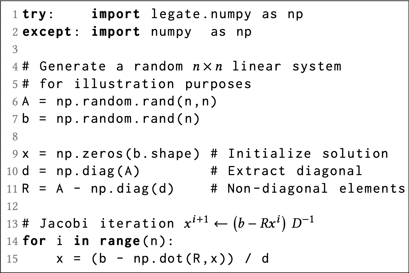
of such work can be found from Nvidia Legate (Bauer and Garland 2019). In the
paper, the authors show how Nvidia CUDA is integrated with
Python’s scientific array programming library called NumPy in a
convenient way, as shown in Fig. 3. Previous
work to Legate also exist in form of CuPy (Okuta et al. 2017) and Numba (Lam, Pitrou, and Seibert
2015). CuPy and Numba compare closely to Legate, but without
inter-device work scheduling.
Sample code showing GPGPU paradigm seamlessly integrated
into Python’s NumPy. (Source: (Bauer and Garland
2019))
Projects like Legate, CuPy, and Numba are a prime example of
performance "lifting" of productivity-focused languages like Python
towards more complete triangles, per the mental model of Fig. 1. Arguably, from the viewpoint of a
developer who is satisfied with Python, the triangle is complete – they
have a) the performance of CUDA (if GPU is present) and b) if not, they
are simply using CPU NumPy (which itself is accelerated with OpenMP on
CPU), and c) they are using a language they feel is general and
productive for them.
Given the possibility for the completeness of abstractions like
Legate, it is no wonder that alternative approaches exist. For example,
there exist GPGPU "lifters" for Matlab-like language Julia (Bezanson et al.
2017). Some programmers may find languages like Julia better
suited for their use-case, as the whole language is built on scientific
computing. In specific, in Julia arrays and matrices as first-class,
whereas in Python, such traits are imported via libraries like
NumPy.
A differentiating take is Futhark (Henriksen et al.
2017) which is a functional programming language with GPGPU as
language built-in feature. Interestingly, Futhark is able to represent
the GPGPUs register-orientated computing paradigm in the functional
programming paradigm, which is presented in the more traditional
non-parallel computing approach. For example, average of a vector in
Futhark is computed with:
let average (xs: []f64) = reduce (+) 0.0 xs / r64 (length xs)
Here, it is worth noticing that the indices which would traditionally
be required in the GPGPU paradigm are abstracted. Furthermore, some may
find a functional programming style preferable over imperative
approaches of Python and Julia.
APL examples here show rank polymorphism on plus operation
over scalar, vector, and matrix. Note that looping is implicit. Also,
note that APL is read right-to-left: definition of the mat is a reshape
of 1..9 vector over the left-hand-side
argument, hence producing 3x3 matrix with values taken from range 1..9.
Another approach to achieve performance for parallel computing is to
make the language the array programming library. A family of languages
that do this is known informally as APLs, which are based on a 1962
paper (Iverson 1962) by Kenneth
Iverson (a recent historical view on the language is provided in (Hui and Kromberg
2020)). In the paper, a language called A Programming Language
for teaching matrix algebra was introduced. An interesting and
distinctive aspect of APLs is that there is no explicit iteration or
recursion in the standard2(“Programming languages —
APL” 1989), but instead, operation ranks are
automatically lifted to higher dimensions. This means that, e.g., plus
operation works irrespective of the array rank, as demonstrated in Fig.
4. It has been argued (Slepak, Shivers, and
Manolios 2014) that such abstraction solves the so-called von
Neumann bottleneck (Backus 1978) which complements
Iverson’s own argument for APL being "a tool of thought" (Iverson 2007).
In abstract, APL proponents call the capability of rudimentary index
operation abstraction as a programming approach that contributes to the
correctness and brevity of computation solving. In other words, as less
effort is put into thinking about programming paradigms, APLs free
attention towards the original mathematical problem on-hand. More
recently (e.g., see: (A. Hsu 2019; Slepak, Shivers,
and Manolios 2014)), APL’s model of loop and recursion-free array
processing has gained research interest as a way to simplify parallel
computation. In specific, in (A. Hsu 2019), a data-parallel compiler
was introduced. Here, it was shown that arrays could be used to
represent abstract syntax trees. The produced compiler (A. Hsu, n.d.), called
co-dfns, is able to produce C, CUDA, and OpenCL code from a
subset of APL when using the proprietary Dyalog APL interpreter. As
such, the project ascends APLs usability to modern-day GPGPU computing. We deem this
as an interesting and fundamental development in terms of performance
implications for GPGPU code: as APL and its
operands amount to simple matrix operations, then by forcing such
array-based problem solving, it would force the developer to write
automatically parallel code. As argued in length in (McKenney
2017), part of the reason parallel code is hard to write is that
developers fail to understand the underlying hardware. As such,
developers may unknowingly produce sequential algorithms and data
structures and cause the hardware to compute redundancies, which slow
computation. Redundancies include, e.g., using branch predictor over
binary selector. According to Nvidia presentation (Harris et al. 2007),
elimination of branch prediction can increase throughput by 2x on
GPUs.
Contribution
High-level overview of the research done in this study, and
how they relate to previous work
With a brief introduction to programming languages and methods of
hardware acceleration for parallel computation covered, we now focus on
this study’s focus. First, we present a high-level overview in Fig. 5.
This figure details how we combine four different aspects (machine
learning, computer networks, high-performance computing, and programming
languages) in two different research branches (AI and systems) by using
software engineering (which itself is a systems science) to produce a
contribution which combines these aspects into one integrated process.
Finally, we show that future work can be done to extend our hereby
presented contribution with theoretical computer science by using logic
and verification.
The context of our study is GPU microservices as a method to
accelerate NFV. We conclude from the
previous research that GPU microservices are a timely subject because:
1) the new Vulkan API and SPIR-V IR can fix interoperability problems of
past GPGPU approaches for microservices and 2) general trend in
computation is towards parallelism and fine-grained programs, for which
GPUs are a good fit for. Further, we decide to tackle the domain with
APL. This is because we notice that fast parallelism is enabled by SIMD, and APL introduces us to
rank polymorphism. With rank polymorphism, APL can transform any
operation to vectors, which may benefit from SIMD. Additionally, APL forces
us to think from an array-only mindset, which may produce unconventional
but highly parallel approaches to solving existing problems. This, in
turn, compliments our guest for new ways to do effective NFV
services by replacing purpose-built digital signal processors with
commodity hardware such as GPUs. With the convoluted problem statement,
we next move onto the empirical part of the study.
The empirical part of the work is a development to (Brissaud et al.
2019), in which RF prediction is used to label
encrypted hypertext data. We use the paper’s application in this study
by extracting the prediction algorithm as a GPU microservice, using the
CPU implementation execution time as the baseline to improve on. We
choose this application also because the binary decision tree traversed
by RF algorithms can be
parallelized as each three is data-independent. Further, the amount of
the trees to traverse is usually well above the amount of normal amount
of logical threads that a CPU may have. As a thesis, such workload
should see performance increase on GPUs, as the GPUs have thousands of
cores. To elaborate, the physical processor of GPU is less likely to get
throttled by its physical capabilities compared to its CPU counterpart,
assuming that the execution time of the program takes long enough time.
Henceforth, when referring to the "RF algorithm," or "our algorithm," we
refer to this Python-based algorithm, which we will translate to SPIR-V
in this study.
As mentioned, our approach to writing the GPU implementation is
unusual: we rewrite the Python implementation in APL and use APL as a
modeling language to write SPIR-V assembly code from. We argue that
hand-writing APL operands in SPIR-V assembly are a worthwhile endeavor:
APL is recently shown to produce well-parallelizable code (A. W. Hsu 2016) and its
domain-specificity in array programming is already the base of modern
machine learning libraries, such as NumPy, which we believe vouches for
APL’s fitness for machine learning acceleration. More importantly, APL
as a language is comprised of only around 60 operations (albeit across
four separate dimensions of scalar, vector, matrix, and cuboid), for
which we deem it practically viable to offer hand-written SPIR-V
implementation for each procedure. Further, we find some evidence that
APL is strict enough to repel programmer constructions that diverge from
parallel computation principles: the side-effects of zealous array
programming, in specific, avoidance of explicit recursion and if-clauses
(i.e., thread divergence), forces the programmer to write performant GPU
code by default.
Yet, as GPUs are not typical computers, implementing all the
operations for a full compiler is not without its eccentricities. As
such, in §3.2, we describe some of the underlying
peculiarities that affect GPUs.
Next, in §3.3.1, we notice that SPIR-V is a useful IR
for another reason: the produced binary files are few kilobytes and can
hence be inlined within text files. We use this finding to propose a way
to orchestrate GPU NFs on Kubernetes using Vulkan
in the following subsections.
Python to APL translation
In this study, we use paper Passive Monitoring of HTTPS Service
Use(Brissaud et al. 2019) as a
case-study. The idea was to reimplement the RF
algorithm used for NFV use-case on GPU.
We decided to use APL as a modeling language. In the end, we
reimplemented three functions in APL:
Here, the third item labels the result received from the second item.
The second item normalizes and sums prediction values received by
traversing the RF trees. The first item is the traversal algorithm of an
RF tree, and coincidentally, it is the most computationally heavy
function. In this study, we only implemented the full GPU
reimplementation of the first item. This was because this function was
the only part of the Python code which had C-optimizations. As such, it
would be the only part which was accelerated in the Python version hence
made a good comparison against a GPU implementation. Next, we describe
our process of reimplementing the Python to APL and then to SPIR-V
IR.
Methodology The debugger with pyCharm IDE was used
to introspect the scikit and numpy models,
from which numpy.savetxt function was used to extract model
files to a .csv file. Using Sourcegraph, the
scikitRF implementation3, 4 was refactored using the
pyCharm debugger to produce APL program which produced the same result.
We used Dyalog 17.1 IDE to test the APL code.
Remarks The APL program is model specific in the
sense that it assumes the user only wants a single result. As such,
there are no guarantees the same program works across all possible RF
models which are compatible with Python. Yet, for the purpose of a
simple case-study, we accept limiting the model output to 1 as fine.
Translation The first call to prediction is in the
h2classifierrf_tools.py file. This file is
part of our Github project5, which remains internal
to Inria for the time being. Nevertheless, the file has a call as
follows:
pred_lab = clf.predict(feat_)
Where clf is our model and feat_ are the
samples. This call forwards to a function like this in:
As our output size is 1, we only have to consider the first
if-clause. But before that, the self.predict_proba(X) calls
the following:
def predict_proba(self, X): check_is_fitted(self)# Check data X =self._validate_X_predict(X)# Assign chunk of trees to jobs n_jobs, _, _ = _partition_estimators(self.n_estimators, self.n_jobs)# avoid storing the output of every estimator by summing them here all_proba = [np.zeros((X.shape[0], j), dtype=np.float64)for j in np.atleast_1d(self.n_classes_)] lock = threading.Lock() Parallel(n_jobs=n_jobs, verbose=self.verbose,**_joblib_parallel_args(require="sharedmem"))( delayed(_accumulate_prediction)(e.predict_proba, X, all_proba, lock)for e inself.estimators_)for proba in all_proba: proba /=len(self.estimators_)iflen(all_proba) ==1:return all_proba[0]else:return all_proba
Here, we focus on the parallel code that Python evaluates,
specifically this block:
Parallel(n_jobs=n_jobs, verbose=self.verbose,**_joblib_parallel_args(require="sharedmem"))( delayed(_accumulate_prediction)(e.predict_proba, X, all_proba, lock)for e inself.estimators_)
The way this call should be interpreted is the following: for each
e in self.estimators_, calls the
_accumulate_prediction function, to which a function
parameter e.predict_proba among normal variables parameters
X, all_proba, and lock are
passed. This brings us to the _accumulate_prediction
function, which looks like this:
Again, we have to only consider the if-clause in which the number of
outputs is one, but before that, the function
self.tree_.predict is called. This brings us to the next
function:
def predict(self, *args, **kwargs): # real signature unknown""" Predict target for X. """pass
Here, we see that the call-stack "disappears" but in fact, this means
we are calling Cython, which is Python-like language which compiles into
platform-specific bytecode. In general, when we install
performance-accelerated libraries like scikit, the fetch
will compile the static libraries for us. To see the actual source code,
we have to clone the un-compiled project. From here, we can see that the
function which is called is the following:
cpdef np.ndarray predict(self, object X):"""Predict target for X.""" out =self._get_value_ndarray().take(self.apply(X), axis=0, mode='clip')ifself.n_outputs ==1: out = out.reshape(X.shape[0], self.max_n_classes)return out
As can be seen, the dialect is now a mix of C and Python. Here,
self._get_value_ndarray() constructs a numpy
presentation of the tree_ object with which we called the
code, which uses the take() method to do the actual RF
model prediction. The constructor looks like this:
cdef np.ndarray _get_value_ndarray(self):"""Wraps value as a 3-d NumPy array. The array keeps a reference to this Tree, which manages the underlying memory. """ cdef np.npy_intp shape[3] shape[0] =<np.npy_intp>self.node_count shape[1] =<np.npy_intp>self.n_outputs shape[2] =<np.npy_intp>self.max_n_classes cdef np.ndarray arr arr = np.PyArray_SimpleNewFromData(3, shape, np.NPY_DOUBLE, self.value) Py_INCREF(self) arr.base =<PyObject*>selfreturn arr
The self.value variable here comes from the following
method:
def __setstate__(self, d):"""Setstate re-implementation, for unpickling."""self.max_depth = d["max_depth"]self.node_count = d["node_count"]if'nodes'notin d:raiseValueError('You have loaded Tree version which ''cannot be imported') node_ndarray = d['nodes'] value_ndarray = d['values'] value_shape = (node_ndarray.shape[0], self.n_outputs,self.max_n_classes)if (node_ndarray.ndim !=1or node_ndarray.dtype != NODE_DTYPE ornot node_ndarray.flags.c_contiguous or value_ndarray.shape != value_shape ornot value_ndarray.flags.c_contiguous or value_ndarray.dtype != np.float64):raiseValueError('Did not recognise loaded array layout')self.capacity = node_ndarray.shape[0]ifself._resize_c(self.capacity) !=0:raiseMemoryError("resizing tree to %d"%self.capacity) nodes = memcpy(self.nodes, (<np.ndarray> node_ndarray).data,self.capacity * sizeof(Node)) value = memcpy(self.value, (<np.ndarray> value_ndarray).data,self.capacity *self.value_stride * sizeof(double))
Here, we can see that the self.value represents the data
that resides within the d["values"] structure. Next, we may
focus on the self.apply(X) call of the initial
predict function, which brings us to the following
function:
cpdef np.ndarray apply(self, object X):"""Finds the terminal region (=leaf node) for each sample in X."""if issparse(X):returnself._apply_sparse_csr(X)else:returnself._apply_dense(X)
Our tree is always dense, so we look at the dense call, which brings
us to this function:
cdef inline np.ndarray _apply_dense(self, object X):"""Finds the terminal region (=leaf node) for each sample in X."""# Check inputifnotisinstance(X, np.ndarray):raiseValueError("X should be in np.ndarray format, got %s"%type(X))if X.dtype != DTYPE:raiseValueError("X.dtype should be np.float32, got %s"% X.dtype)# Extract input cdef const DTYPE_t[:, :] X_ndarray = X cdef SIZE_t n_samples = X.shape[0]# Initialize output cdef np.ndarray[SIZE_t] out = np.zeros((n_samples,), dtype=np.intp) cdef SIZE_t* out_ptr =<SIZE_t*> out.data# Initialize auxiliary data-structure cdef Node* node = NULL cdef SIZE_t i =0with nogil:for i inrange(n_samples): node =self.nodes# While node not a leafwhile node.left_child != _TREE_LEAF:# ... and node.right_child != _TREE_LEAF:if X_ndarray[i, node.feature] <= node.threshold: node =&self.nodes[node.left_child]else: node =&self.nodes[node.right_child] out_ptr[i] =<SIZE_t>(node -self.nodes) # node offsetreturn out
This is now the bottom function of the call stack. We focus on the
with nogil: part and everything that comes after it, as
this is the parallel code we are looking for. Informally, what happens
here is the following: first, the nogil notation is a
pragma to OpenMP acceleration library which releases the global
interpreter lock of Python. Essentially, this is required for the code
to run fast. Inside of the pragma, we find that we iterate each sample
in our tree, and then do a binary selection on it. If the node in the
sample is TREE_LEAF, which is a constant of
-1, then we save the previous node index into a Cython
pointer structure. Once we return the function, we should have a
collection of indices which the Cython predict function
then uses to take values out of the initial tree model. It is worth
noticing that the node = self.nodes points to a
Node type. This is given earlier in the source code:
This is an important remark because the Node structure
is another layer of abstraction: it creates relations between different
nodes and the tree’s decision tree. This can be slightly misleading. For
example, let us first consider an APL candidate to replace the decision
tree traversal:
To do the translation, we first assume that
node = self.nodes refers to both the array’s address and
its contents, as typical in C. Next, we note that APL is read right to
the left. Next, we can assume the index of 1 to be the
first parameter in the APL node definition. After this, the
APL uses a dfns while construct. The loops conditional
is:
⍵⌷left≠¯1
Here, we check whether the value of the left array at omega is
-1. Omega is the right-hand side parameter identifier in
APL, which here amounts to one, per the reasoning in the previous
paragraph. Next, if the conditional is true, then
⍵{⍵+1⌷,right[⍺;],left[⍺;]}i(⍵⌷feature+1)⌷x≤⍵⌷th
Here, the code has two blocks, of which
i(⍵⌷feature+1)⌷x≤⍵⌷th
Is executed first. Here, we take the variable i, which
amounts to the for loop’s index, as in the Cython code. We then use
clauses to calculate the index at omega on the feature array and add 1
to it to fix a compatibility issue with Python indexing (in Python,
index 0 is the first value, whereas in APL it is 1). These two calls
mean that we make a selection of row i and column
⍵⌷feature+1 of x array, which is the sample
array. We then compare the result with the one at position omega on
array th (threshold). The omega here is the index passed
from the right-hand side, that is, it is the value 1. Now,
the call
i(⍵⌷feature+1)⌷x≤⍵⌷th
Will print either 0 or 1, corresponding to False or True. This is
then passed into the second part of the APL call:
⍵{⍵+1⌷,right[⍺;],left[⍺;]}
Here, we have first placed omega of the outer block (that is, the
value of 1) as the alpha argument (left-hand side) to go inside the
bracketed call. We do this because the binary value from the above call
will get passed as the omega argument inside the bracketed call. The
call itself makes a selection: it adds 1 to the binary value and uses
this value to make a selection between the two arrays. This means it
retrieves either the value at position alpha from the array
right when the comparison call received False or
alternatively the position alpha from the array left when
the comparison was True. The resulting value will then be returned as
the omega parameter back to the while condition. Once false, the while
loop terminates, and the previous value will be saved in the call
out[i]←node
Where the i is the loop iterator value, and the node is
the last loop value from the while. As an example, assume that the
binary selection is always True, and the left array is
(2 3 -1 4). Now, we would first pluck 2 from
the array and use the index to find the second value from the left array
again, assuming that the binary selection always returns 1.
We would then get 3, which gets looped again because it is
not -1. On the third iteration, we would find
-1 after which we would return from the loop, and have the
value 3 as the node value. In a usual case, we would bounce
between the right and left arrays until we
would find -1.
Yet, the APL implementation is slightly incorrect as APL starts
indexing from 1. To fix this, we modify the code to follows:
This is now the RF tree traversal code refactored to APL. As the main
point, we see that traversing the RF tree requires explicit recursion.
This is a bad sign, as it is telling us that the operation within it
cannot be parallelized in APL. In general, we would assume that in this
point the data structure has to be transformed to something such as a
parallel tree structure (i.e., see [cite]) for better performance, but
in this case, we retain the original approach of the Python code to
better compare CPU against GPU.
Next, we move up in the call stack back to the Python functions. The
APL equivalent of everything is:
{{1⌷[2]↑⍒¨↓⍵(÷⍤1 0){⍵+0÷⍵}+/⍵}⍵}
What we have here is a sum reduction +/⍵ applied to a
normalization ⍵(÷⍤1 0){⍵+0÷⍵}, after which for each matrix
column a descending indices sort is applied ⍒¨↓, and the
indices of each column are returned 1⌷[2]↑.
In general, it could be said that in Python, much effort goes into
dealing with asynchronous and parallel code, which requires multiple
methods, source files, and libraries. In APL, these performance
improvement methodologies are implicit, and the math function of the RF
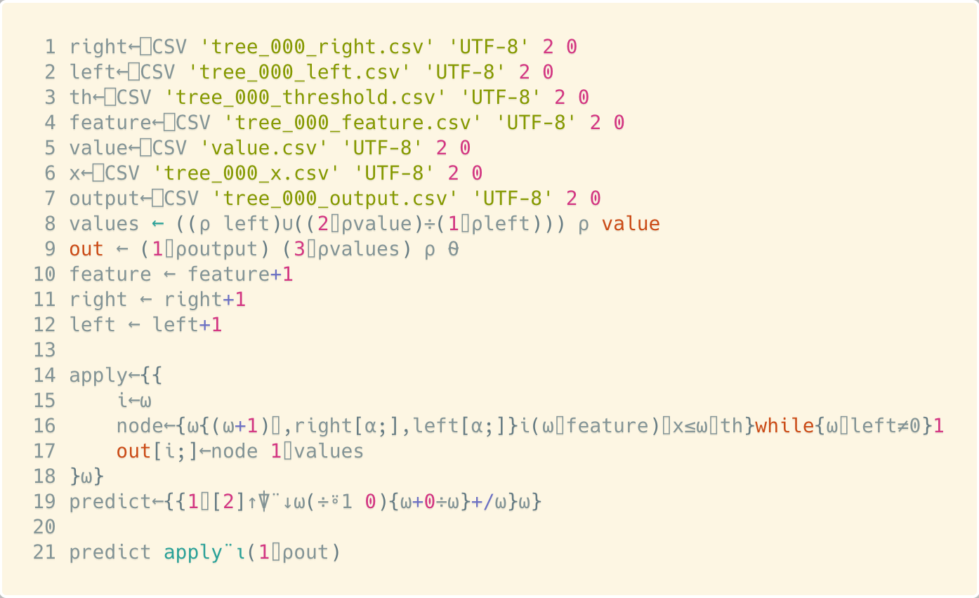
prediction is arguably more succinctly described. In essence, the APL
code produced at this time can be written in seven lines of code, as
shown in the Appendix.
As for the SPIR-V code, the final product is found in the Appendix.
In the SPIR-V code, we used the APL implementation rather than the
Python implementation as the reference. The translation itself is
rudimentary, with the idea being that in future work, these hand-coded
translations would be generated as the program output whenever a given
operation is used. Since APL only has a limited amount of operations, an
APL-SPIRV compiler amounts "only" to the implementation of the supported
mathematical operations. As such, given a complete APL operand support,
generating executables equals to correctly interpreting APL calls to
produce the main function, which calls the manually coded SPIR-V.
Regarding novelty, its not exactly a proper compiler, but the GPU
targeting produces enough quirks and pitfalls to keep things interesting
(see: 3.2).
Further, we saw that hand-writing SPIR-V code enabled some novelty:
on line 99, the SPIR-V IR stores a pointer representing an array of 198
values in a single assignment. This is interesting because the current
cross-compilers for GLSL and MSL
are unable to do so. As such, the only way to do such an operation with
the current SPIR-V tooling is to write it by hand. We believe this
vouches for the usefulness of a direct SPIR-V target output in future
work.
Programming in SPIR-V
During our research, we made an effort to translate Python to APL to
SPIR-V. During this time, we learned about the details of SPIR-V, which
we have documented in the following chapters.
Subgroup operations
Whilst GPUs have many threads, SIMD operations are not automatically
applied. Instead, similar to AVX programming, separate instructions must
be used. On GPUs and SPIR-V hence Vulkan in specific, such operations
are called group operations. Group operations historically abstracted
away so-called workgroup level operations, but nowadays, the
best-practice is to use a more refined class of instructions belonging
to subgroup operations6, which is as a named concept
specific to SPIR-V (i.e., Nvidia calls subgroup operations as "warps").
On the SPIR-V specification, the subgroup operations are listed under
3.36.24. Non-Uniform Instructions7.
The usefulness of subgroup operations is that the opcodes abstract the
manufacturer-specific approaches to do SIMD operations on each kind of
GPU, mobile or desktop. As a historical reference to the avid reader, to
understand more about subgroup operations, we found online resources
Vulkan Subgroup Explained8 and Optimizing
Parallel Reduction in CUDA9 the most helpful.
Because of the parallel hardware design, some operations are trickier
on GPUs than on CPUs. E.g., let us consider a reduce operation on a CPU.
In the functional programming paradigm, a reduce operation could be
described as a recursive function on a vector of natural numbers: the
last element of the vector is summed to the previous element until the
vector length is one. In principle, the sum operation should, therefore,
apply to any non-empty vector.
On GPUs, it is possible, albeit extraordinarily inefficient, to use
the same principle. This is because GPUs launch a workgroup per
a compute unit of a GPU, which then each hold invocations which
handle parallel tasks. As explained with an example in §2.2.2, GPUs essentially hold a thread for
each element of the vector, and the program structure must be defined
from the viewpoint of a single thread (i.e., invocation). As an
added complexity, in SPIR-V, unless the size of the vector is coded in
the program source, it is to our understanding impossible10
to define the length of the vector at runtime. Such constraints are very
rarely considered in CPU algorithms, which forces us to fundamentally
rethink many of our approaches.
Yet, neither is managing memory without its peculiarities: an
invocation cannot share stack memory with invocations in other
subgroups. Heap memory allocation during runtime is also
impossible. This means that it is impossible to declare a function-local
variable and compare it to the values of other invocations unless the
two invocations reside within the same subgroup. In this sense, a
subgroup resembles an AVX SIMD-lane – register values beyond the single
SIMD lane are not accessible, and the width of the SIMD lane is
dependent on the physical attributes of the hardware. In our tests, we
noticed that Nvidia GPUs tend to have a subgroup width of 32 registers
and AMD GPUs with a width of 64. Further, in some cases, the width can
change during runtime. However, these registers are very efficient.
Indifferent to CPU AVX instructions, which are restricted by the
byte-width of the register (e.g., AVX-512 supports 512-bit registers),
the registers on GPU are not dependent on the size of the value in the
register. This means that it is possible to fit a 4x4 float matrix on a
single register on GPU, and as such, do arithmetic on 64x4x4 registers
(on AMD) using a single operation call without accessing the slow
uniform-class memory storage.
But beyond subgroup sizes, communication between invocations must be
done via shared heap memory, which must hold a particular visibility
scope11 which are an important concept for
performance. Heap-based communication also requires explicit
synchronization: changes in the heap are not visible to pointer
references automatically, but instead, must be synchronized via
memory barriers, which synchronize the state across programmer
specified visibility Scope. Hence, understanding memory
barriers and memory synchronization are required for space-efficient
computation, and to avoid non-determinism. Further, session-based
synchronization primitives, prevalent in concurrent programming
languages, such as channels in Go and D, are not available. Instead,
changes in the heap memory are managed either by 1) atomic operations of
integer and floating-point types or 2) via the Vulkan memory model. Yet,
there exists an exception to this regarding our use-case in machine
learning workloads for the Vulkan memory model, which does not support
atomic operations on floats. A number of machine learning applications
deal with probabilities hence require floating-point representation.
This means that compute kernels like ours, which use the Vulkan memory
model in part to understand more about Vulkan but also to support even
the most recent opcodes, are excluded from inter-thread communication
via atomic operations. Instead, the pointer-based Vulkan memory model
via memory barriers must be used instead.
Vulkan memory model
The Vulkan memory model is formally verified, open-source12 specification to ensure
well-founded memory management for GPUs. The Vulkan memory model is
written in Alloy (Jackson 2019), which is a model
checker designed to find bugs in parallel and asynchronous software. As
GPUs are parallel computers, ensuring correct ordering of memory
accesses is paramount to avoid non-deterministic results. Further, the
Vulkan memory model is deemed novel: according to the Khronos Group, the
open industry consortium responsible for both the Vulkan graphics API
and the SPIR-V IR language, the Vulkan memory model is "the world’s
first graphics API with a formal memory model." 13
Relevant to our study, two concepts of the Vulkan memory model,
Availability and Visibility, are important. We focus
on these concepts as they are, as defined above, the only memory
operations that support interthread communication on floating-point
numbers, relevant to our case-study of RF prediction algorithm. And
as the Vulkan memory model was mainlined into the SPIR-V specification
in the version 1.5, which was released on September 13th, 2019, we also
deem it relevant contribution to documenting our understanding and usage
of it – previous academic work regarding the use of these memory
primitives for compute kernels seem non-existent, likely due to the
recency of the specification.
Regarding the definition of the terms, according to a blog post by
Khronos14, "Availability operations ensure
that values written to a memory location in one thread can be made
available to other threads. Visibility operations guarantee that values
which are available are made visible to a thread, to ensure that the
correct values are read. For typical devices supporting Vulkan,
availability and visibility operations will map to cache control (e.g.,
flushes/invalidates/bypass)." The blog post continues to detail some
general usages, of which to us the most relevant is the Read-after-Write
usage, as it models the interthread communication between invocations in
different subgroups. According to the blog post, when a pointer is read
after writing, it requires the writer to be first made available and
then visible before the read. In practice, per the SPIR-V documentation
on memory operands15 this means that for memory operands
which modify shared data, we must apply
MakePointerAvailable or MakePointerVisible
flag when calling OpStore or OpLoad operand,
respectively. The specification also specifies that these flags have to
be accompanied by an additional flag of NonPrivatePointer,
which defines that the memory access obeys inter-thread ordering. After
the flags, a memory scope identifier is also required. The scope
identifier allows the specification of how "far" the pointer operation
will trickle in the memory domain. This is useful for performance: the
memory bandwidth, according to a blog post which benchmarked subgroup
operations against threadgroups16, even for thread
groups, which are higher-order memory abstraction than subgroups, hence
slower, maybe up to 10x faster than global memory, and the latency for
memory access for thread groups is up to 40x faster than for global
memory. On the other hand, the same blog post also remarks that it might
be harder to use subgroup operations than workgroup or global memory
operations. In this case, we found it to be the opposite when writing
SPIR-V by hand: thread group operations were not supported by our
hardware, while subgroup operations were, and semantically there is no
difference in SPIR-V whether data is loaded and stored from a subgroup,
thread group, or global memory. In this light, we remark that writing
SPIR-V by hand, i.e., instead of using cross-compilers, enables easier
usage of the new performance-improving primitives. Alas, this improved
control over performance does not come free: writing SPIR-V code, which
is an intermediate representation, after all, is much more laborsome
than, say, existing shader languages like GLSL
or MSL.
The bottom line is that computation on the GPUs is tricky for memory
reasons: both memory storage and memory communication requires
understanding GPU-specific concepts. What follows is that also, many
classical algorithms do not work as-is on GPUs. Yet, for the sake of the
focus of this research, further considerations for optimal algorithms or
their correct implementations are left for future research. As will be
seen in the following sections, a lot of systems understanding is
required merely to bootload GPU programs.
Orchestration of GPU compute resources
An envisioned software stack of a GPU node.
Similar to previous NFV approaches, such as
Netbricks (Panda
et al. 2016), in this study, our microservice architecture
leverages Rust programming language. Further, also similar to Netbricks,
we run the NFs unvirtualized. Here, we
leverage low-level Vulkan API bindings to allow us to
refine the GPU computation pipeline to accustom to performance. To
elaborate, we declare static resources that exist along the complete
lifetime of the program, with other parts, such as program loading,
working in a dynamic manner (see: left side of Fig. 9). Next, to allow GPU NFs to be
orchestrated, we integrate our Rust-loader application with Kubernetes
Service abstractions (see: Fig. 8). In
particular, the novelty of our approach here comes from the fact that
SPIR-V kernels can be inlined within Kubernetes Service abstraction as
string-valued metadata. This is possible because SPIR-V kernels are
small in size: our RF prediction algorithm weights in at 2kb without
compression. Furthermore, we achieve a non-virtualized and non-container
approach while still managing to leverage Kubernetes APIs by defining
the GPU nodes inherently as non-schedulable (by not having CRI
installed, see: Fig. 7) and the Service abstractions as services
without selectors. This way, we achieve two things: 1) Kubernetes does
not try to schedule any existing worker nodes (for software stack, see:
Fig. 6) to spawn containers for the GPU
Services as the Service declarations lack selectors, and 2) the Services
are still exposing as a cluster-wide DNS entry. This keeps our
proposed approach non-invasive to existing Kubernetes installations.
Hence, we believe that our proposal to orchestrate GPU NFs this way can
be practically viable. The major benefit of integrating with the
standard Kubernetes scheduling workflow, orientated around the Service
abstraction, is that the GPU Services in our proposed architecture is
automatically seen, routed, and exposed within the cluster as any other
standard container-based service. This way, we can heavily simplify our
loader program: CNI handles the networking,
CoreDNS the routing, and etcd the kv-storage. For example, for better
networking performance, CNI integrations like Cilium can be used to
automatically benefit from kernel-passthrough technology BPF.
Such an approach might be useful when running the GPU NFs on the edge of
the network, providing even lower latency to data inference or simply to
gain higher packet throughput. The following subsections are meant to
further detail and visualize our proposed approach.
Kubernetes Integration
As mentioned, Kubernetes (Burns et al. 2016) is an orchestrator
system for containers, and can be considered as a system which
conglomerates multiple physical servers into a single abstracted
computing unit. Kubernetes is designed to schedule software packaged
into containers, but due to its modular design, it can be retrofitted to
also serve other purposes. In this study, we propose a way to retrofit
Kubernetes to orchestrate GPU microservices in a cluster, which can also
do containers in the traditional way. As such, we consider our approach
"non-invasive", as we do not limit the functionality of the standard
installation.
Kubernetes integration. Here, four instances form the
Kubernetes abstraction. Green instances are container-schedulable, the
red one is not.
Due to Kubernetes’ modular design, the architecture of each
installation may vary. In our study, we propose a barebone installation
without making too many assumptions about what the underlying modules
are. To illustrate our idea, we consider a network topology of a
four-node system, in which we have one primary node and three
secondaries (pictured in Fig. 7). Here, of the
three secondaries, two of them are container hosts, whereas one of them
is a GPU host. We propose that the GPU host remains non-schedulable for
containers, per arguments regarding NF performance (e.g., see (Panda et al.
2016)). On the cluster level, we do not simply cordon the GPU
hosts, but instead, never install a CRI on the host. This is a
possible solution when the Kubernetes cluster installation is done
manually (e.g., per instructions of (Hightower, n.d.)). However, even though the
GPU instance is unuseful hence in a sense redundant for the cluster for
running containers, it may still be part of the cluster as long as it
has the CNI installed properly. The
CNI is just another module on the Kubernetes stack and can be, e.g.,
flannel or something else. The CNIs then rely on
etcd which is a distributed kv-storage and one of the most
basic requirements for a Kubernetes instance. We insist on the fact that
in our proposed architecture, the CNI, CRI and the GPU host operating
system may be whatever, as the software stack does not need to be
opinionated thanks to the modular interface provided by Kubernetes (to a
stark difference, e.g., in Legate (Bauer and Garland 2019) where the
software stack must be based on proprietary Nvidia stack).
Once these basic services are installed on each node, they should
provide a DNS layer for proper addressing withing the cluster. Usually,
this is done via CoreDNS as it has a Kubernetes integration, but may
also be some other DNS server. Relevant to our proposal, the DNS server
is required to correctly route Kubernetes Services, which is the main
interface our proposed architecture needs. To quote the Kubernetes
documentation, a Service is "an abstraction which defines a logical set
of Pods and a policy by which to access them (sometimes this pattern is
called a micro-service)". In other words, Service is the
Kubernetes-native way of defining a microservice. As such, it is logical
for our proposal on the orchestration of GPU NFs as microservices to
interface with the Service abstraction.
Kubernetes Service declarations. On the left, one with
selectors, which would spawn container image MyApp. On the right, a
Service without a selector, which would not spawn any containers. Our
proposal uses the right-hand side version to spawn GPU NFs as
microservices.
Yet, we do not use the standard declaration of Service, because we do
not want to run the GPU NF microservices inside of a container. To
elaborate, using containers for GPU applications is tricky and
opinionated. For reference, the Kubernetes documentation on using GPUs17 lists that to use, e.g., Nvidia
GPUs, the cluster has to: 1) have Nvidia drivers pre-installed, 2) have
nvidia-docker installed (which only works on Linux), 3) use Docker as
the CRI. For AMD, the steps include similar tweaks, including allowing
the nodes to run in a privileged mode. In essence, these approaches
limit the flexibility of the GPU node installations and require
dangerous execution modes for containers, which are usually meant to run
in an unprivileged mode. We note that in our proposal, drivers still
have to be installed, in addition to Vulkan, but our proposal allows the
GPU nodes to remain operating system and CRI agnostic. We achieve this
by declaring the Service abstraction without a node selector. To compare
these declarations, consider Fig. 8. Further, for
the Service not to remain orphan, we must declare an Endpoint
abstraction manually. This can be done in a single command by separating
the configuration declarations with three dashes, as shown in Fig. 8.
As can be seen on Fig. 8, our proposal for declaring GPU
microservices within Kubernetes requires the SPIR-V binary file to be
inlined within the metadata description. In our initial proposal, we do
not compress the binaries, and the binaries are encoded in base64. Also,
the binding count has to be included, which defines how many buffers the
SPIR-V kernel includes. The buffers in our initial proposal are always
defined as Vulkan Storage Buffers with the Compute type.
After the creation of the Service file, CoreDNS triggers a CNAME
entry creation for the Service. We clarify that this is a standard
procedure in Kubernetes, which is automatically triggered on Service
creation. By default, this would expose an endpoint by name
my-service.default.svc.cluster.local in each of the
cluster’s nodes’ routing table. In our proposal, what follows is that
the Service creation events would be listened by the GPU nodes using a
Kubernetes client-wrapper, e.g., kube-rs. This means that
each GPU node is listening to the primary Kubernetes node to announce
changes in the cluster Service entries. One such is found, the GPU nodes
would pull the declarations using the HTTP API. This would reveal the
SPIR-V binary encoded in base64 and the number of buffer bindings that
have to be created for this particular GPU microservice. Finally, if the
Endpoints include the node-local IP address, the microservice is
provisioned using the Vulkan API. Once the microservice is initialized,
the according to port found in the Service declaration is opened on the
node. When the port receives packets, the contents are unmarshaled to 1D
vector array buffers in Rust and passed to GPU. Once done, the result is
written back to the connection which it came from. As such, it is the
responsibility of the Kubernetes CNI to route data in and out. Such
reliance cuts two ways: on the one hand, our proposal only works with
Kubernetes. But on the other hand, we do not make assumptions about what
the Kubernetes installation has to be like. As such, it is possible to
leverage Kubernetes abstractions on top of the GPU NFs, such as
LoadBalancer, to balance the load among many GPU nodes or any other
networking constructs. For example, to create a function-chain of NFs,
we would encourage the chaining to be declared on Kubernetes-level. This
way, the function-chain may mix both GPU NFs and CPU NFs by interfacing
via CNAME entries. As such, we consider that our proposal can be used to
introduce GPU NFs and other microservices as part of a heterogeneous
system consisting of CPU and GPU nodes.
Vulkan-based Loader Program
Our Vulkan-based loader program (see: 9 and
high-performance computing and software engineering level contribution
on 5) uses a Rust-wrapper library called
ash18 to interface with the GPU. In the
abstract, ash provides conveniences, e.g., wrapping
returned structures in vectors, and providing default values for all API
call structures. It is also a very low-level in the sense that all
operations are "unsafe", which essentially means that the programmer
must consult the official Vulkan API documentation to avoid undefined
behavior. Coincidentally, this means that the Rust compiler is less
useful than usually in respect of memory safety: unsafe calls are meant
as code blocks in which the programmer surpasses the type system, and
everything in ash is unsafe.
In Fig. 9 we demonstrate the program flow of the
loader. We start from declaring static variables, i.e., ones which
extend to the complete lifetime of the program. Once these are
initiated, the shader modules and pipeline layouts of the shaders are
retrieved from Kubernetes using a Rust client library to Kubernetes
called kube-rs19. This could be
considered as analogous to pulling a container image from a registry to
be ready-to-deploy. After this initialization, we open the ports
specified by the Kubernetes Services and start waiting for input to the
kernels. Once input is received, it goes through a standard Vulkan
compute pipeline, which we have detailed step-by-step in the
aforementioned figure. In the final step, once the result is copied back
to CPU memory, the result is written back to the network socket
specified by the Kubernetes Service file. Here on, it is the job of
Kubernetes CNI to forward the response to wherever. As such, it could be
argued that this way, our approach yields itself well to the working
principles of chained NFs, allowing such constructs to be modeled in
Kubernetes, possibly spanning multiple Services with GPU NFs and
traditional CPU containers complementing each other. Further, we yield
to the fact there should exist more performant ways to traverse the
Vulkan pipeline – understanding Vulkan to use it in the most effective
way is a subject of many books, thus effectively out-of-scope of what
could have been prepared for this study. As such, further pipeline
optimizations are left for future studies.
Vulkan loader in a nutshell.
Results
Runtime comparison of random forest model of 150x6000x300
trees between Cython and SPIR-V.
The benchmarks were run on an Intel i7 processor and Nvidia GTX 2080
GPU. As introduced previously, the application was a RF
prediction over 150x6000x300 dimensional trees (i.e., quite small). As
shown in Fig. 10, the Cython code on OpenMP was faster
than the GPU code: the average runtime of the Cython code was 380ms (8
cores, 6000 threads) while the SPIR-V took on average 480ms (1024 cores)
to execute. Further, the performance variance on the GPU was higher than
on the Cython code.
However, even though the GPU code was slower, we estimate that there
exists future work in making the GPU approach faster. In specific, due
to the time limits of our research, each data buffer is copied
separately to the GPU. While the dataset is not big (our dataset weights
in at 70MB in total), the memory copies happen sequentially. Yet, it is
possible to use Vulkan’s fine-grained performance primitives to
structure the data in such a way that a single memory copy would
suffice. Similarly, garbage collection of the Vulkan resources could be
done asynchronously, whereas currently, the operations block each tree
iteration. Furthermore, the data structure of the binary decision tree
could be reformatted into a path matrix (A. W. Hsu 2016). Such a parallel data
structure would allow the GPU to use its y-dimension cores when
traversing the tree.
Altogether, we think these results are promising. GPUs are oftentimes
thought to only be practical approach after a certain threshold is met,
but here we show it can be almost comparable to CPU performance even for
small datasets.
Discussion and Future Work
In our case-study in Section §3 we
relied on a hand-coded SPIR-V program. But what about compiling APL
straight to SPIR-V and automatically creating the Kubernetes manifest
files? According to our research, such is possible but does not come
without its challenges. First, the problem considers the well-researched
subject of the static compilation of APL. We found that as of recent,
the matter has been studied in (Slepak, Shivers, and Manolios 2014)
(2014). It seems the work continues with two new pre-prints appearing in
2019 (Slepak,
Shivers, and Manolios 2019; Shivers, Slepak, and Manolios 2019).
In abstract, these papers introduce a new language that leverages
dependant types to achieve static rank polymorphism. Meanwhile, in (Gibbons
2017) argument is made against inventing a new language. In (Gibbons
2017), the author argues for using Haskell to implement a type
checker for static rank polymorphism and provides proof that the issue
of type checking APL is possible given the current state of programming
language theory and its tools.
Next, we detail why the type checking is important in the context of
our goals: one unique challenge GPU environments introduce over the CPU
is the non-existence of shared stack memory and inability to allocate
memory at runtime. As such, for a generic compiler, the compiler would
need to infer the intermediate types after each operation step until
program termination. Interestingly, this would also imply that the
problem touches on so-called static memory management, which has been an
issue in recent programming language research (e.g., (Proust 2017)). To
elaborate on the problem, let us suppose the following program:
⍒ 4 4 ⍴ ?⍳16
which produces depending on randomness, e.g.,
3 4 2 1
I.e., create a random list of 16 integers, reshape them into 4x4
matrix, and for each row of the matrix, sum the values together, and
rank then according to the sum value from highest to lowest.
When this program is given to the loader program, the problem is that
the buffer dimensions inferred from the initial argument (index of) 16
are not relevant considering the output (of shape 4). This is a problem
because the output buffer has to be allocated prior to program
execution, meaning that, what would be loaded from the GPU memory would
be: 3 4 2 1 0 0 0 0 0 0 0 0 0 0 0 0. This is a false result and would
need to be either reshaped on the GPU or the CPU, but regardless of
which hardware it is done, the type inference (more precisely in APL
terms, the shape inference) has to be known prior to the execution of
the kernel (to clear out the unneeded numbers). Yet, the only way to
know the final shape of the array is to make a type of inference of the
whole program as most APL interpreters are made for CPU hardware they do
not concern type inference prior to the runtime as they are able to
allocate shared stack memory.
In addition, because of the rho which transforms the list of 16
numbers into a 4x4 matrix, which is then graded down using the indices
sort function, we are also introduced to an intermediate problem: the
sorting needs to be applied to a shared matrix (as sorting is
data-dependant on other threads values), but the matrix has no physical
mapping, nor is it the output of the program. To our current knowledge,
there are two apparent options to handle this:
Infer the matrix transformation prior to execution and allocate
an "intermediate" physical global work buffer Q, which is given as the
target memory to the reshape function. This would mean that there are
three memory allocations: one for the input (1x16, class CPU-GPU), one
for the reshape (4x4, class GPU-only), and one for the output (1x4,
class GPU-CPU). Now, the reshape would map the memory into a 4x4
device-class storage buffer, which could then be manipulated using the Y
dimension invocation identifier. Hence, this would mean that the Y
dimension of the workgroup should always be at least the maximum of any
intermediate shapes’ Y dimension.
Infer the matrix transformation prior to execution, and either
allocate or use any "old" memory buffer layouts (memory buffers which do
not hold any data-dependency to forthcoming executions) to fit the data
into. In this example, the input buffer (1x16, class CPU-GPU) would fit
our whole matrix if laid into a one-dimensional format. Also, the input
buffer has served its purpose (the program does not need it anymore), so
the memory in there would be safe to overwrite. Now, the reshape would
map the memory by using a stride identifier of 4. This means, that even
though the matrix is handled in a one-dimensional array, the SPIR-V
would keep an additional variable in-memory to know that depending on
the X dimension invocation identifier, that it is not supposed to use
the indices sort beyond the stride. For example, if the invocation ID is
14, this ID could be divided by the stride to infer the "logical" Y
dimension of the array. As a benefit, the stride could be coded as a
function-local variable within the compilation, hence saving access or
allocation in global memory. So, with this approach, it would mean that
there are two memory allocations: one for the input (1x16, class
CPU-GPU), and one for the output (1x4, class GPU-CPU). The memory usage
has decreased, but this method would two-step of one very complicated
thing: identify orphan memory + use it such that it can fit the memory
(what about if the orphan memory is 3x10? it fits but not exactly,
requires more complex stride logic).
Yet, the 2) is logically an improvement over the 1), and 1) would be
required at all times: if there simply will not be eligible orphan
memory, or it is too small, then memory allocation should be inferred to
the principle of 1).
However, this is good to think as it relates closely to the way the
information is fed to the GPU: even though it would be possible to
define input buffers to already adhere to a matrix or vector dimensions,
it might be limiting (and slowing) factor if the original memory layout
is probed to be re-used.
A second aspect that would improve from the application of computer
science theory is the memory safety of the programs. The more
complicated the APL operands become, the more error-prone it is to prove
that the algorithms do what they are supposed: GPU programs are parallel
constructs, and hence may act nondeterministically. This act is further
complicated by the way the memory has to be handled as pointers in the
program state – pointers are generally known to be a very error-prone
concept. We stipulate that in the future the APL operands of which the
compiler stitches together should either be verified with a model
checker to avoid concurrency bugs, or, e.g., use some form of separation
logic to make sure that certain parts of the program hold
invariants.
As the bottom line, we deem it interesting to next apply proper
computer science logic to our contribution: the arguably at-times hacky
approach to combine many aspects of system sciences together in this
study seems to be ripe to be improved by formalism next. Further, it may
well be that due to relation with high-performance computing, the
results found in later studies might be practically viable, especially
given the fact that should the aforementioned Kubernetes approach be
presented as a software plugin rather than mere textual description.
Conclusion
This study was conducted in the context of NFV, which seeks to
replace purpose-built network hardware with commodity hardware such as
GPUs. In this study, we used rank polymorphic programming language APL
as a parallel modeling language for SPIR-V IR GPU code. In general, we
studied how APL could work as a compiled GPU DSL for NFV. Hence, we
introduced a way to deploy GPU code written this way to Kubernetes. We
also benchmarked an NFV ML application: we timed RF tree prediction of
size 150x6000x300 between CPU and GPU. We found that OpenMP powered
Cython code on CPU was, on average, 26% faster than our hand-written
Vulkan SPIR-V GPU code. We remark that the benchmark does favor the CPU
over GPU due to the small size of the RF tree. We also suggest
performance improvements to our GPU implementation. We also discuss
challenges and opportunities for extending the APL DSL with type
inference. As a conclusion, given the groundwork done in this study, we
consider such future work prosperous. In specific, future work would
provide novel yet practical features to NFV via ease of programming and
verifiable memory consumption policies.
Full APL code
APL refactor of the Python source code.
Due to the font-problems of LaTeX, we present the multiline
source-code of APL as Fig. 11 instead of
textual representation.
Agache, Alexandru, Marc Brooker, Alexandra Iordache, Anthony Liguori,
Rolf Neugebauer, Phil Piwonka, and Diana-Maria Popa. 2020.
“Firecracker: Lightweight Virtualization for Serverless
Applications.” In 17th {USENIX}
Symposium on Networked Systems Design and Implementation ({NSDI}
20), 419–34.
Amaral, Marcelo, Jorda Polo, David Carrera, Iqbal Mohomed, Merve Unuvar,
and Malgorzata Steinder. 2015. “Performance Evaluation of
Microservices Architectures Using Containers.” In 2015 IEEE
14th International Symposium on Network Computing and Applications,
27–34. IEEE.
Backus, John. 1978. “Can Programming Be Liberated from the von
Neumann Style? A Functional Style and Its Algebra of Programs.”Communications of the ACM 21 (8): 613–41.
Bauer, Michael, and Michael Garland. 2019. “Legate NumPy:
Accelerated and Distributed Array Computing.” In Proceedings
of the International Conference for High Performance Computing,
Networking, Storage and Analysis, 1–23.
Bezanson, Jeff, Alan Edelman, Stefan Karpinski, and Viral B Shah. 2017.
“Julia: A Fresh Approach to Numerical Computing.”SIAM
Review 59 (1): 65–98.
Brissaud, Pierre-Olivier, Jérôme Francçis, Isabelle Chrisment, Thibault
Cholez, and Olivier Bettan. 2019. “Transparent and
Service-Agnostic Monitoring of Encrypted Web Traffic.”IEEE
Transactions on Network and Service Management 16 (3): 842–56.
Brown, Kevin J, Arvind K Sujeeth, Hyouk Joong Lee, Tiark Rompf, Hassan
Chafi, Martin Odersky, and Kunle Olukotun. 2011. “A Heterogeneous
Parallel Framework for Domain-Specific Languages.” In 2011
International Conference on Parallel Architectures and Compilation
Techniques, 89–100. IEEE.
Burns, Brendan, Brian Grant, David Oppenheimer, Eric Brewer, and John
Wilkes. 2016. “Borg, Omega, and Kubernetes.”Queue
14 (1): 70–93.
Fouladi, Sadjad, Riad S Wahby, Brennan Shacklett, Karthikeyan Vasuki
Balasubramaniam, William Zeng, Rahul Bhalerao, Anirudh Sivaraman, George
Porter, and Keith Winstein. 2017. “Encoding, Fast and Slow:
Low-Latency Video Processing Using Thousands of Tiny Threads.” In
14th {USENIX} Symposium on Networked Systems Design and
Implementation ({NSDI} 17), 363–76.
Gibbons, Jeremy. 2017. “APLicative Programming with Naperian
Functors.” In European Symposium on Programming, 556–83.
Springer.
Haas, Andreas, Andreas Rossberg, Derek L Schuff, Ben L Titzer, Michael
Holman, Dan Gohman, Luke Wagner, Alon Zakai, and JF Bastien. 2017.
“Bringing the Web up to Speed with WebAssembly.” In
Proceedings of the 38th ACM SIGPLAN Conference on Programming
Language Design and Implementation, 185–200.
Haavisto, Juuso, Muhammad Arif, Lauri Lovén, Teemu Leppänen, and Jukka
Riekki. 2019. “Open-Source RANs in Practice: An over-the-Air
Deployment for 5G MEC.” In 2019 European Conference on
Networks and Communications (EuCNC), 495–500. IEEE.
Haavisto, Juuso, and Jukka Riekki. 2020. “Interoperable GPU
Kernels as Latency Improver for MEC.” In 2020 2nd 6G Wireless
Summit (6G SUMMIT), 1–5. IEEE.
Han, Sangjin, Keon Jang, KyoungSoo Park, and Sue Moon. 2010.
“PacketShader: A GPU-Accelerated Software Router.”ACM
SIGCOMM Computer Communication Review 40 (4): 195–206.
Harris, Mark et al. 2007. “Optimizing Parallel Reduction in
CUDA.”Nvidia Developer Technology 2 (4): 70.
Hellerstein, Joseph M, Jose Faleiro, Joseph E Gonzalez, Johann
Schleier-Smith, Vikram Sreekanti, Alexey Tumanov, and Chenggang Wu.
2018. “Serverless Computing: One Step Forward, Two Steps
Back.”arXiv Preprint arXiv:1812.03651.
Henriksen, Troels, Niels G. W. Serup, Martin Elsman, Fritz Henglein, and
Cosmin E. Oancea. 2017. “Futhark: Purely Functional
GPU-Programming with Nested Parallelism and in-Place Array
Updates.” In Proceedings of the 38th ACM SIGPLAN Conference
on Programming Language Design and Implementation, 556–71. PLDI
2017. New York, NY, USA: ACM. https://doi.org/10.1145/3062341.3062354.
Hsu, Aaron W. 2016. “The Key to a Data Parallel Compiler.”
In Proceedings of the 3rd ACM SIGPLAN International Workshop on
Libraries, Languages, and Compilers for Array Programming, 32–40.
Hui, Roger KW, and Morten J Kromberg. 2020. “APL Since
1978.”Proceedings of the ACM on Programming Languages.
Imada, Takayuki. 2018. “Mirageos Unikernel with Network
Acceleration for Iot Cloud Environments.” In Proceedings of
the 2018 2nd International Conference on Cloud and Big Data
Computing, 1–5.
Iverson, Kenneth E. 1962. “A Programming Language.” In
Proceedings of the May 1-3, 1962, Spring Joint Computer
Conference, 345–51.
———. 2007. “Notation as a Tool of Thought.” In ACM
Turing Award Lectures, 1979.
Jackson, Daniel. 2019. “Alloy: A Language and Tool for Exploring
Software Designs.”Commun. ACM 62 (9): 66–76. https://doi.org/10.1145/3338843.
Jangda, Abhinav, Donald Pinckney, Yuriy Brun, and Arjun Guha. 2019.
“Formal Foundations of Serverless Computing.”Proceedings of the ACM on Programming Languages 3 (OOPSLA):
1–26.
Jonas, Eric, Johann Schleier-Smith, Vikram Sreekanti, Chia-Che Tsai,
Anurag Khandelwal, Qifan Pu, Vaishaal Shankar, et al. 2019. “Cloud
Programming Simplified: A Berkeley View on Serverless Computing.”arXiv Preprint arXiv:1902.03383.
Kratzke, Nane. 2017. “About Microservices, Containers and Their
Underestimated Impact on Network Performance.”arXiv Preprint
arXiv:1710.04049.
Lam, Siu Kwan, Antoine Pitrou, and Stanley Seibert. 2015. “Numba:
A Llvm-Based Python Jit Compiler.” In Proceedings of the
Second Workshop on the LLVM Compiler Infrastructure in HPC, 1–6.
Lattner, Chris, Mehdi Amini, Uday Bondhugula, Albert Cohen, Andy Davis,
Jacques Pienaar, River Riddle, Tatiana Shpeisman, Nicolas Vasilache, and
Oleksandr Zinenko. 2020. “MLIR: A Compiler Infrastructure for the
End of Moore’s Law.”https://arxiv.org/abs/2002.11054.
McKenney, Paul E. 2017. “Is Parallel Programming Hard, and, If so,
What Can You Do about It?(v2017. 01.02 a).”arXiv Preprint
arXiv:1701.00854.
Okuta, Ryosuke, Yuya Unno, Daisuke Nishino, Shohei Hido, and Crissman
Loomis. 2017. “Cupy: A Numpy-Compatible Library for Nvidia Gpu
Calculations.” In Proceedings of Workshop on Machine Learning
Systems (LearningSys) in the Thirty-First Annual Conference on Neural
Information Processing Systems (NIPS).
Panda, Aurojit, Sangjin Han, Keon Jang, Melvin Walls, Sylvia Ratnasamy,
and Scott Shenker. 2016. “NetBricks: Taking
the V out of NFV.” In 12th USENIX
Symposium on Operating Systems Design and Implementation (OSDI
16), 203–16.
“Programming languages — APL.”
1989. Standard. Vol. 2006. International Organization for
Standardization.
Proust, Raphaël L. 2017. “Asap: As Static as Possible Memory
Management.” University of Cambridge, Computer Laboratory.
Raza, Ali, Parul Sohal, James Cadden, Jonathan Appavoo, Ulrich Drepper,
Richard Jones, Orran Krieger, Renato Mancuso, and Larry Woodman. 2019.
“Unikernels: The Next Stage of Linux’s Dominance.” In
Proceedings of the Workshop on Hot Topics in Operating Systems,
7–13.
Shivers, Olin, Justin Slepak, and Panagiotis Manolios. 2019.
“Introduction to Rank-Polymorphic Programming in Remora
(Draft).”https://arxiv.org/abs/1912.13451.
Slepak, Justin, Olin Shivers, and Panagiotis Manolios. 2014. “An
Array-Oriented Language with Static Rank Polymorphism.” In
European Symposium on Programming Languages and Systems, 27–46.
Springer.
Watt, Conrad. 2018. “Mechanising and Verifying the WebAssembly
Specification.” In Proceedings of the 7th ACM SIGPLAN
International Conference on Certified Programs and Proofs, 53–65.